In this article
I built a ray-tracing pipeline in CorneaForge to calculate how measured corneal surfaces bend light. It follows rays through the front and back of the cornea, measures their optical paths, and expresses the differences with Zernike coefficients. This connects the geometry we acquire to the optical behavior we want to describe.
The calculation brings together interpolation, differential geometry, numerical optimization and linear algebra inside the Python engine used by CorneaForge and OphtaFlow AI. Each method has a concrete job: locate the surface, find its orientation, bend a ray, find its next intersection, and summarize the resulting wavefront.
A surface changes a ray through its slope
Start with parallel rays traveling toward the eye. At the cornea, each ray meets a differently tilted patch of surface. The patch’s orientation determines the change in direction.
Write the surface height as z = f(x, y). Its gradient, (∂f/∂x, ∂f/∂y), describes how quickly the height changes along each horizontal coordinate. From these two slopes, I construct a normal: a vector perpendicular to the surface.
For light traveling along positive z, I orient the normal toward the incoming light:
N = (∂f/∂x, ∂f/∂y, −1)
n̂ = N / ||N||
The division gives n̂ length one. At the center of a symmetric surface, both slopes vanish and the normal points directly against the incoming ray. Away from the center, it tilts.
Real measurements arrive at discrete locations. I implemented this optical path using a bicubic spline, a smooth piecewise polynomial surface, on the polar sampling grid. Its derivatives supply the slopes between observations. SciPy’s bivariate spline implementation evaluates both heights and derivatives. I convert the radial and angular derivatives into Cartesian slopes before constructing the normals.
Refraction is a vector calculation
The refractive index, n, measures how much a medium slows light relative to vacuum. At a boundary, Snell’s law relates the incoming and outgoing angles, measured from the normal:
n₁ sin(θ₁) = n₂ sin(θ₂)For the corneal calculation, I use indices of 1.000 for air, 1.376 for the cornea and 1.336 for the aqueous humor, the fluid behind it. The first boundary bends light toward the normal; the second changes its direction again.
A ray arriving from air at 30° from the normal enters the cornea at about 21.3°. That smaller angle is the bending toward the normal.
In three dimensions, I apply Snell’s law directly to unit vectors. Let i be the incoming direction, n̂ the surface normal pointing against it, and η = n₁/n₂:
c = −i · n̂
t = η i + (ηc − √(1 − η²(1 − c²))) n̂
Here · is a dot product and t is the transmitted direction. The square root supplies the cosine of the transmitted angle. This established construction is also explained in Physically Based Rendering’s treatment of refraction.
I vectorized the calculation with NumPy: positions, directions and normals are arrays with one row per ray. A batch of dot products and elementwise operations refracts the whole bundle.

Find where the ray reaches the second surface
After the first refraction, a ray travels obliquely through the cornea. Its posterior intersection must lie on both the ray and the back surface.
Let A be its anterior intersection and t its direction inside the cornea. Any point along it can be written as:
P(s) = A + s tThe unknown distance s must also satisfy Pz(s) = f_back(Px(s), Py(s)). On a measured surface represented by a spline, I solve the intersection numerically.
I implemented Newton iteration to refine that intersection. Each correction uses the local surface slopes to bring the candidate point closer to the ray and the posterior surface together.
Inside the Newton step
With a = tₓ/tz and b = tᵧ/tz, the three errors to drive to zero are:
r₁ = x − Ax − a(z − Az)
r₂ = y − Ay − b(z − Az)
r₃ = z − f_back(x, y)
The first two keep the point on the ray. The third places it on the posterior surface. At each iteration, the Jacobian, the matrix of derivatives of these errors, gives a linear correction:
J ΔP = −r
P_next = P + ΔP
I solve these small systems across the ray bundle and track convergence per ray. Once an intersection is found, the posterior slopes give a new normal, and a second application of Snell’s law sends the ray into the aqueous humor.
Curvature changes the focus
A tighter anterior curve turns the rays more strongly. Decrease the anterior radius in this two-dimensional spherical example and watch the focus of a near-axis ray move. Its displayed distance starts at the posterior vertex. Distances are in millimeters; the posterior surface and refractive indices stay fixed.
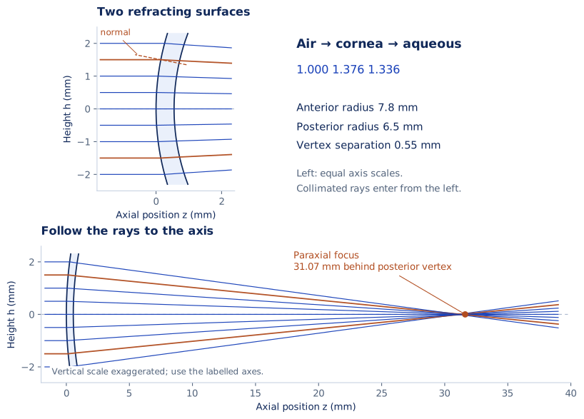
Near-axis focal distance: 31.07 mm from the posterior vertex.
Posterior radius 6.5 mm; vertex separation 0.55 mm. Air 1.000 → cornea 1.376 → aqueous 1.336. Height is in mm, enlarged ×2.5 in the interactive view.
The full engine traces a three-dimensional bundle across an analysis disk. Rays from different parts of a surface generally do not meet at exactly one point. I estimate a focal location by least squares: find the position and depth that minimize their transverse spread. The remaining differences carry information about the optical system.
Measure the path in optical units
Optical path length weights each traveled distance by the refractive index of its medium. For our three segments:
OPL = n_air d_air + n_cornea d_cornea + n_aqueous d_aqueousA millimeter inside a material contributes more optical path than a millimeter in air. This weighting connects geometric distance to the phase accumulated by light.
The endpoint convention matters. In my implementation, each outgoing ray ends on a plane perpendicular to that ray and passing through the estimated focal point F. If Q is its posterior intersection and t its outgoing unit direction, the final distance is:
d_aqueous = |(F − Q) · t|I then subtract the bundle’s mean optical path:
OPDᵢ = OPLᵢ − mean(OPL)This optical path difference, or OPD, tells us how each ray differs from the bundle’s common reference. Removing the mean eliminates a constant offset while preserving differences across the aperture.
Turn optical differences into coefficients
Now the calculation returns to the Zernike fitting problem. Each retained ray has a position in the analysis disk and an OPD value. I evaluate the normalized Zernike basis at those positions and solve:
choose c to minimize ||A c − OPD||²I fit 36 terms through radial order 7 and express the coefficients in micrometers. Astigmatism, coma and spherical aberration occupy different modes. The square root of the sum of squared coefficients from radial order 3 upward gives the higher-order aberration root mean square (RMS), a compact measure of those components.
The engine evaluates diameters from 2 to 7 mm with both pupil and corneal-vertex centering. Its total-cornea output removes piston, the constant mode, and defocus, the mode associated with focus, after fitting; the anterior-only output removes piston. These choices define what the exported coefficient vector contains.
Put the physics inside the feature pipeline
I integrated these computations into the shared feature profiles used for device-file processing and model inference. Surface splines are built once and reused across apertures and centers, applying the same reuse principle as the geometry cache to a different numerical calculation.
The resulting features describe optical effects with explicit surfaces, indices, apertures and references. I can also change the question: how much comes from a regular fitted shape, and how much remains after it is removed? That leads to choosing a reference surface, where I compare geometric models and trace their contribution to the residual.