In this article
A residual map shows the difference between a measured surface and a chosen reference. Change the reference, and the same measurements produce a different map.
I built conoid and biconic fitting into CorneaForge to make that choice part of the computation. Each fit produces a compact description of the broad surface shape, then a residual describing what that model leaves behind. I designed these research descriptors to retain both parts of the explanation.
The useful question is what each reference absorbs. A model that captures directional curvature removes it from the residual; a rotationally symmetric model leaves some of it visible. That distinction reaches all the way into the features supplied to an ML model.
One surface, two explanations
Consider a constructed surface over a disk of radius 2 mm. It has different curvatures along its horizontal and vertical directions, plus a small off-center bump:
z(x, y) = x² / (2 Rx) + y² / (2 Ry) + bump(x, y)

Rx = 7 mm, Ry = 9 mm
The bump is a Gaussian centered at (0.8, 0.4) mm, with a width of 0.35 mm. Its default height is 20 µm. These are constructed inputs chosen to separate a broad directional shape from a local feature.
I fit two simple references to exactly the same points:
Axisymmetric:  z_ref = a₀ + a₁(x² + y²)
Anisotropic:   z_ref = b₀ + b₁x² + b₂xy + b₃y²
Axisymmetric means unchanged by rotation around the center. Anisotropic means the shape can depend on direction. These quadratic models provide a local illustration of the reference choice; the conoid and biconic implementations below use fuller surface equations.

The axisymmetric fit has only one quadratic curvature coefficient. It must compromise between the two directions, leaving a broad pattern around the bump. The anisotropic fit can explain that directional background, changing both the residual pattern and its overall magnitude.
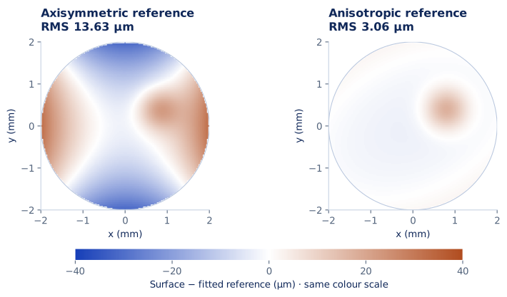
Residual RMS: 13.63 µm.
Residual range: −31.21 to +32.31 µm.
Surface minus fitted reference, on a 2 mm radius disk. The quadratic surface keeps the same directional curvature; the slider changes only its local bump. Both fits use the same points and colour scale.
Set the bump height to zero. The anisotropic model can then recover the constructed surface exactly, to numerical precision. Increase the bump again: the broad fit also absorbs part of that local feature, because every sampled point participates in the fit.
Both views use the same color scale. The displayed root mean square, or RMS, is sqrt(mean(residual²)) over the sampled disk. It summarizes remaining height differences in micrometers. A smaller RMS tells us that this reference explains more of these points; interpreting that change requires knowing what it explained.
Choose the family before fitting its parameters
A sphere describes a surface with constant curvature. A conic surface of revolution adds an asphericity parameter, usually written Q, which controls how the profile departs from a sphere away from the apex. Both remain rotationally symmetric around their own axes.
A toric reference introduces different principal curvatures in two perpendicular directions. A biconic additionally allows separate conic constants in those directions. A quadric is an implicit surface described by a second-degree polynomial in three coordinates; its ellipsoidal form provides the conoid representation used in my implementation.
These families make different shape assumptions. They are not interchangeable names for a smooth fit. Corneal fitting with directional curvature and asphericity has a substantial history, including Langenbucher, Viestenz and Seitz’s conoidal fitting work and the later biconic fitting method of Janunts, Kannengießer and Langenbucher.
I implemented separate conoid and biconic paths because their parameters distribute shape differently between the reference and the residual.
Turn a quadric into a solvable system
For the conoid path, I start with valid native surface points expressed in millimeters. The fitted equation is:
a₁₁x² + a₂₂y² + z² + a₁₂xy + a₁₃xz + a₂₃yz
    + b₁x + b₂y + b₃z + c = 0
Fixing the coefficient of z² to one leaves nine unknowns. Although the equation contains squared coordinates, it is linear in those unknown coefficients. Each observed point supplies one row of a matrix:
design = np.column_stack([
    x*x, y*y, x*y, x*z, y*z, x, y, z, np.ones_like(x)
])
coefficients, _, _, _ = np.linalg.lstsq(design, -(z*z), rcond=None)
This minimizes squared errors in the implicit equation: an algebraic fit. It does not directly minimize vertical height differences or shortest distances to the surface. I therefore evaluate the resulting surface at the measured (x, y) positions and calculate height residuals separately.
That distinction matters when comparing algorithms. “Least squares” names an objective structure; the quantity being squared still determines what the solver favors.
Recover axes from the coefficients
The quadratic terms form a symmetric matrix A, so the equation becomes:
pᵀ A p + bᵀ p + c = 0Here p is the three-dimensional position. I find the center by solving A p₀ = −b/2, then use NumPy’s symmetric eigendecomposition. Its eigenvectors identify the principal directions; its eigenvalues determine the quadratic scaling along them.
For an accepted ellipsoid, those scales give semi-axis lengths. Writing them as s₁, s₂, and s₃, with the third axis identified as the depth direction, my extraction includes:
Rx = s₁² / s₃          Ry = s₂² / s₃
Qx = s₁² / s₃² − 1     Qy = s₂² / s₃² − 1
The shared s₃ couples the two directions. This is a concrete restriction of the conoid parameterization.
A shallow surface patch can also constrain the fitted heights better than the orientation of the enclosing ellipsoid. I chose to compute residuals in the original instrument coordinates, evaluating the quadric there. The exported conoid features retain geometry and fit diagnostics; the eigenvector-derived orientation fields are excluded from that output.
Give the biconic its own objective
The biconic path fits eight parameters: two radii, two independent conic constants, a height offset, an in-plane orientation, and two tilt terms. The implementation models tilt with a first-order height correction.
Here the minimized residual is directly z_measured − z_biconic. I implemented bounded nonlinear least squares using SciPy’s trust-region reflective solver, initializing from the conoid where available. The bounds constrain the parameter search. The output includes the height RMS and a conditioning diagnostic that reports how unevenly the observations constrain parameter changes.
This is a separate fit with a different surface family and objective, so its result deserves its own name and parameters.
Keep both halves of the description
After fitting, I decompose the residuals into 45 Zernike terms through radial order 8, retaining coefficients alongside reference parameters and fit errors. The Zernike article explains how the sampled least-squares decomposition works. This path uses measured height minus reference height; the sign must travel with the descriptor.
For ML, the useful representation can include both halves: the broad shape absorbed by the reference, and the variation left behind. Keeping only the residual would discard information deliberately assigned to the reference. Choosing the lowest residual RMS alone would reward that removal without asking whether the removed information matters to the prediction task.
Comparisons also need the same analysis region and sampling rule. This demonstration weights a Cartesian grid uniformly; the implementation works from native polar samples. Those are different distributions of observations over the disk.
The residual can become a rendered map with cached interpolation or a coefficient vector. For the optical decomposition, I trace the measured surface and its fitted conoid separately, then compare their optical path differences using a shared focal reference. In From corneal shape to light, I follow surface geometry into ray tracing. Across those representations, the reference remains part of the result: it records which shape the calculation has already explained.